Mathematical Modeling with Python (JijModeling)
In this section, you will learn how to formulate the Job Shop Scheduling Problem and implement the model using Python.
Python Environment Setup Procedure
First, here are the recommended Python environment setup steps for using JijZept SDK.
Using a virtual environment helps prevent dependency conflicts and maintains a clean development environment.
For JijZept IDE Users
In the JijZept IDE environment, Python and package setup is not required. You can start the tutorial right away.
For details, please refer to the JijZept IDE documentation.
Python Environment Setup
- Create a virtual environment
Terminal window python -m venv .venv - Activate the virtual environment
Terminal window source .venv/bin/activate - Install JijZept SDK
Terminal window pip install "jijzept_sdk[all]"This command installs all packages needed for the optimization tutorial, including JijModeling, OMMX, and MINTO.
- Install analysis and visualization packages
Terminal window pip install pandas matplotlib
What is JijModeling: Concept Introduction
JijModeling is a library for intuitively and declaratively describing mathematical optimization problems using Python. It is designed to allow not only mathematical optimization experts but also software engineers and data scientists to express mathematical formulations as natural Python code.
The main role of JijModeling is to convert optimization models (decision variables, objective functions, constraints) described in a human-readable form into a format that computers (optimization solvers) can interpret. This eliminates the need to manually handle complex formulas and makes it easier to build, validate, and reuse models.
Features of JijModeling
- Declarative description: You can focus on describing "what" you want to optimize (objective function) and "under what" conditions (constraints), without having to worry about the specific solution algorithm ("how" to solve it).
- Clarity and reusability: The structure of the model becomes clear in the code, making it easier to debug, modify, and apply to other problems.
- Integration with the JijZept ecosystem: Models described with JijModeling seamlessly integrate with saving and sharing in OMMX format and executing optimization calculations with MINTO.
In this section, you will learn the basic usage of JijModeling and master how to express optimization problems in code. The existing JijModeling tutorial also serves as a detailed reference, but this tutorial provides step-by-step explanations and examples along the learning path.
Basic Usage: Defining Variables, Objective Functions, and Constraints
Let's look at the basic steps for building an optimization model using JijModeling. Below, we explain how to define parameters, decision variables, objective functions, and constraints. For detailed usage, please refer to the JijModeling Tutorial.
import jijmodeling as jm
# --- Parameter definition (example: weight vector) ---w = jm.Placeholder("w", ndim=1) # 1-dimensional variablev = jm.Placeholder("w", ndim=1) # 1-dimensional variableN = w.len_at(0, latex="N") # Length of w (len(w[0])) displayed as N
# --- Decision variable definition (1-dimensional binary, integer, continuous variables) ---x = jm.BinaryVar("x", shape=(N,)) # Binary variable (shape=(N,))y = jm.IntegerVar("y", shape=(N,), lower_bound=0, upper_bound=1000) # Integer variable (0 to 1000) (shape=(N,))z = jm.ContinuousVar("z", shape=(N,2), lower_bound=0, upper_bound=10) # Continuous variable (0 to 10) (shape=(N,2))
# --- Index definition ---i = jm.Element("i", belong_to=(0, N)) # Index i ranging from 0 <= i < N
# --- Problem definition (maximization) ---problem = jm.Problem("sample_problem", sense=jm.ProblemSense.MAXIMIZE)
# --- Objective function definition ---problem += jm.sum(i, v[i] * x[i])
# --- Constraint definition ---# Example 1: Σ_i w[i] * x[i] <= 5problem += jm.Constraint("select_limit", jm.sum(i, w[i] * x[i]) <= 5)# Example 2: For all i, x[i] <= 2problem += jm.Constraint("sum_constraint", x[i] <= 2, forall=[i])
Formulation and Implementation of the Parallel Job Shop Scheduling Problem
Formulation
First, let's formulate the Parallel Job Shop Scheduling Problem.
Below are the corresponding objective function, constraints, and decision variables.
| Objective Function | Constraints | Decision Variables |
|---|---|---|
| Minimize the makespan (time to complete all jobs) |
|
|
Formulating in accordance with this table, we get the following:
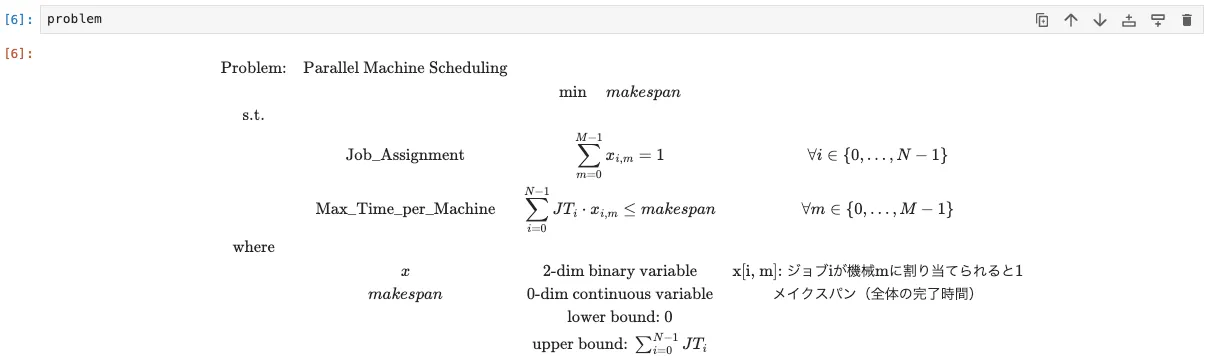
Mathematical Model of the Parallel Job Shop Scheduling Problem
- Decision Variables:
- $x_{im}$: Binary variable that is 1 if job $i$ is assigned to machine $m$, and 0 otherwise
- $makespan$: Maximum completion time of all machines (objective function to be minimized)
- Objective Function:
- $\min makespan$
- Constraints:
- Each job is assigned to exactly one machine:
\[\sum_{m=0}^{M-1} x_{im} = 1,\ \forall i\]
- The processing time $JT_{i}$ of each machine is less than or equal to the makespan:
\[\sum_{i=0}^{N-1} {JT}_i x_{im} \leq makespan,\ \forall m\]
- Each job is assigned to exactly one machine:
Implementation with JijModeling
Let's implement the above mathematical model in Python using JijModeling. Here's an example code:
import jijmodeling as jm
# --- 1. Placeholders (input data) ---# JT[i]: Processing time of job iJT = jm.Placeholder("JT", ndim=1, description="Processing time of job i")# N: Number of jobs (automatically obtained from the length of JT)N = JT.len_at(0, latex="N", description="Number of jobs")# M: Number of machinesM = jm.Placeholder("M", description="Number of machines")
# --- 2. Indices ---i = jm.Element("i", belong_to=(0, N), description="Job index")m = jm.Element("m", belong_to=(0, M), description="Machine index")
# --- 3. Decision variables ---# x[i, m]: Whether job i is assigned to machine m (binary)x = jm.BinaryVar(    "x",    shape=(N, M),    description="x[i, m]: 1 if job i is assigned to machine m")# makespan: Maximum completion time of all machinesmakespan = jm.ContinuousVar(    "makespan",    lower_bound=0,    upper_bound=jm.sum(i, JT[i]),    description="Makespan (total completion time)")
# --- 4. Problem definition ---problem = jm.Problem("Parallel Machine Scheduling")
# --- 5. Constraints ---# Each job must be assigned to exactly one machineproblem += jm.Constraint(    "Job_Assignment",    jm.sum(m, x[i, m]) == 1,    forall=i,)# The total processing time of each machine is less than or equal to the makespanproblem += jm.Constraint(    "Max_Time_per_Machine",    jm.sum(i, JT[i] * x[i, m]) <= makespan,    forall=m,)
# --- 6. Objective function ---# Minimize the makespanproblem += makespan
As shown above, you can formulate a mathematical model using JijModeling with a feeling similar to writing mathematical equations.
If you are using a Notebook or JijZept IDE, you can render mathematical formulas by displaying variable names.