Solving with Solvers (OMMX, JijZept Solver)
In this section, we will define instance data to pass to the mathematical model and explain the process of solving it.
Defining Instance Data
In the previous chapter, we defined a model for the Parallel Job Shop Scheduling Problem using JijModeling. At that time, we defined specific data such as job processing times and the number of machines using Placeholders. Let's now give concrete values to these Placeholders. We define the instance data as a Python dictionary as follows:
# Define instance data# Example: 10 jobs with their respective processing timesjob_times_data = [5, 8, 3, 6, 9, 4, 7, 5, 2, 8]# Example: 3 machines are availablenum_machines_data = 3
# Prepare the data in the dictionary format required by JijModeling Placeholdersinstance_data = {    "JT": job_times_data,    "M": num_machines_data,}
Next, we combine this data with the mathematical model created in the previous chapter to create a specific instance. We use JijModeling's Interpreter to generate an instance with concrete values for the Placeholders.
# 1. Create an Interpreter to evaluate the problem with specific instance datainterpreter = jm.Interpreter(instance_data)# 2. Evaluate the problem to create a concrete instance for the solverinstance = interpreter.eval_problem(problem)The instance created here is represented in a mathematical optimization format called OMMX.
What is OMMX: Purpose and Benefits
OMMX (Open Mathematical prograMming eXchange) is an open standard file format for representing mathematical optimization models, as well as an SDK for manipulating them. It was developed to save and share optimization problems created with modeling tools like JijModeling in a common format that is not dependent on specific tools or languages.
Main Features of OMMX
- Interoperability: By converting models created with JijModeling to OMMX format and then converting them for use with various solvers, it facilitates smooth collaboration between solver tools.
- Persistence: The ability to save optimization models as files (.ommx) makes it easy to reuse them later or share them with other users.
- Sharing and Collaboration: The standardized format makes it easy to share optimization models within teams or between organizations and work collaboratively.
- Tool Independence: Since the model definition is not tied to a specific modeling tool, it can flexibly accommodate future tool changes or the use of multiple tools simultaneously.
Solving with Solvers
Now, let's look at an example of solving the created instance using OMMX. Here, we show how to solve it using JijZept Solver, one of the mathematical optimization solvers, from the OMMX format. This can be done with just the following two lines of code.
import jijzept_solversolution = jijzept_solver.solve(instance, solve_limit_sec=2.0)These two lines of code do the following:
- Pass the OMMX format instance to JijZept Solver to solve it.
- After a solution is obtained, retrieve the solution from the OMMX format instance.
Now, let's look at the results. We can extract the solution from the OMMX solution as follows:
import pandas as pd
optimal_makespan = solution.objectiveprint(f"--- Solver Results ---")print(f"Optimal Makespan: {optimal_makespan:.2f}")assignment = {}  # {machine_idx: [job_idx, ...]}assigned_jobs_flat = (    [])  # To store data for DataFrame: [{'Job': i, 'Machine': m, 'Time': t}]x_result = {}
x_result = solution.extract_decision_variables("x")
# Process the extracted x_result dictionarynum_machines_instance = instance_data["M"]for indices, val in x_result.items():    # indices should be a tuple like (i, m)    if len(indices) == 2 and val > 0.5:  # Check for binary '1'        i, m = indices  # Unpack the indices        if m not in assignment:            assignment[m] = []        assignment[m].append(i)        # Ensure job index i is valid before accessing JT        if 0 <= i < len(instance_data["JT"]):            assigned_jobs_flat.append(                {"Job": i, "Machine": m, "Time": instance_data["JT"][i]}            )        else:            print(                f"Warning: Invalid job index {i} found in solution variable 'x' for machine {m}."            )
print("Job Assignments per Machine:")if assignment:    for m_idx in range(num_machines_instance):        assigned_jobs = sorted(assignment.get(m_idx, []))        print(f"  Machine {m_idx}: Jobs {assigned_jobs}")else:    # This case might occur if x_result extraction failed or was empty despite optimal objective    print("  No assignments could be extracted from 'x' variables.")
# Display assignments clearly using a Pandas DataFrameif assigned_jobs_flat: assignment_df = pd.DataFrame(assigned_jobs_flat) print("Assignment Details (DataFrame):") print( assignment_df.sort_values(by=["Machine", "Job"]).reset_index( drop=True ) )else: print("Assignment Details (DataFrame): Empty")--- Solver Results ---Optimal Makespan: 19.00
Job Assignments per Machine: Machine 0: Jobs [5, 7, 8, 9] Machine 1: Jobs [0, 1, 3] Machine 2: Jobs [2, 4, 6]
Assignment Details (DataFrame): Job Machine Time0 5 0 41 7 0 52 8 0 23 9 0 84 0 1 55 1 1 86 3 1 67 2 2 38 4 2 99 6 2 7# Import plotting libraries if not already doneimport matplotlib.pyplot as pltimport numpy as npimport pandas as pd # For the DataFrame display (assuming done in Sec 9)
num_machines_instance = instance_data["M"]num_jobs_instance = len(instance_data["JT"])job_times = instance_data["JT"] # Alias for convenience
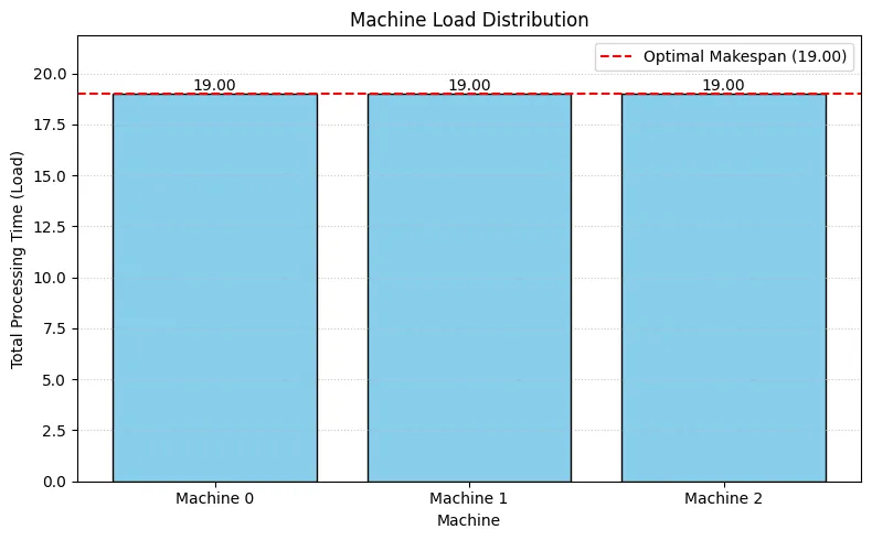
# --- Analysis: Calculate Machine Loads ---print("--- Result Analysis ---")print("Total Processing Time (Load) per Machine:")machine_loads = {m: 0 for m in range(num_machines_instance)}machine_load_list = [] # To store loads for plotting and verification
# Calculate loads directly from the 'assignment' dictionaryfor m_idx in range(num_machines_instance): load = 0 assigned_job_indices = assignment.get(m_idx, []) for job_idx in assigned_job_indices: if 0 <= job_idx < len(job_times): load += job_times[job_idx] else: print( f"Warning: Invalid job index {job_idx} found for machine {m_idx} during load calculation." ) machine_loads[m_idx] = load machine_load_list.append(load) print(f" Machine {m_idx}: {load:.2f}")
# --- Verification ---calculated_max_load = max(machine_load_list) if machine_load_list else 0print(f"Calculated Maximum Machine Load: {calculated_max_load:.2f}")print(f"(Solver's Optimal Makespan: {optimal_makespan:.2f})")# Use a small tolerance for float comparisonif abs(calculated_max_load - optimal_makespan) < 1e-6: print("-> Verification successful: Makespan matches the maximum machine load.")else: print( "-> WARNING: Makespan does NOT match the calculated maximum load. Check model/solver." )
# --- Visualization 1: Bar chart of machine loads ---print("--- Visualization ---")plt.figure(figsize=(8, 5))machines = [f"Machine {m}" for m in range(num_machines_instance)]bars = plt.bar(machines, machine_load_list, color="skyblue", edgecolor="black")plt.axhline( optimal_makespan, color="red", linestyle="--", label=f"Optimal Makespan ({optimal_makespan:.2f})",)
for bar in bars: yval = bar.get_height() plt.text( bar.get_x() + bar.get_width() / 2.0, yval, f"{yval:.2f}", va="bottom", ha="center", )
plt.xlabel("Machine")plt.ylabel("Total Processing Time (Load)")plt.title("Machine Load Distribution")plt.legend()plt.grid(axis="y", linestyle=":", alpha=0.7)plt.ylim(0, optimal_makespan * 1.15)plt.tight_layout()plt.show()
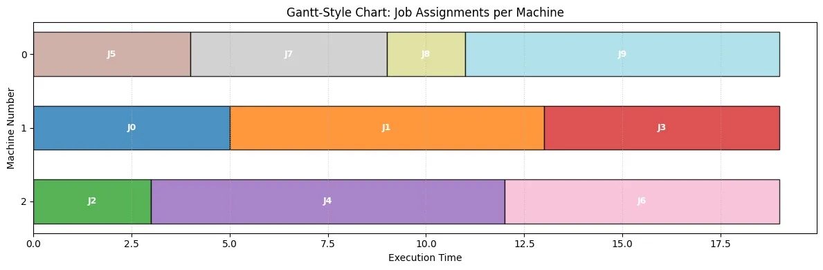
# --- Visualization 2: Gantt-Style Chart of Assignments ---# This chart shows the jobs assigned to each machine sequentially.# The horizontal axis represents time.# Based on the user-provided snippet's logic.
fig, ax = plt.subplots(figsize=(12, max(4, num_machines_instance * 0.8)))# Track the current end time for each machinemachine_end_times = np.zeros(num_machines_instance)job_colors = plt.cm.get_cmap("tab20", num_jobs_instance) # Distinct colors for jobs
print("Generating Gantt-style assignment chart...")
# Iterate through machines and the jobs assigned to themfor m_idx in range(num_machines_instance): # Get assigned jobs for this machine, sort for consistent plotting (optional) assigned_job_indices = sorted(assignment.get(m_idx, []))
for job_idx in assigned_job_indices: if 0 <= job_idx < len(job_times): job_time = job_times[job_idx] start_plot_time = machine_end_times[m_idx]
# Plot the bar for the job ax.barh( m_idx, job_time, left=start_plot_time, height=0.6, align="center", color=job_colors(job_idx % job_colors.N), edgecolor="black", alpha=0.8, )
# Add job index text inside the bar # Adjust text position slightly for better visibility text_x = start_plot_time + job_time / 2.0 text_y = m_idx # Vertically center within the bar's height ax.text( text_x, text_y, f"J{job_idx}", va="center", ha="center", color="white", fontweight="bold", fontsize=9, )
# Update the end time for this machine machine_end_times[m_idx] += job_time else: # This condition should ideally not be met if extraction worked print( f"Skipping plotting for invalid job index {job_idx} on machine {m_idx}" )
# --- Configure plot appearance ---ax.set_xlabel("Execution Time")ax.set_ylabel("Machine Number")# Set y-ticks to match machine indicesax.set_yticks(range(num_machines_instance))ax.set_yticklabels( [f"{m}" for m in range(num_machines_instance)]) # Label ticks with machine numbersax.set_title("Gantt-Style Chart: Job Assignments per Machine")
# Improve appearanceax.invert_yaxis() # Show Machine 0 at the topplt.grid(axis="x", linestyle=":", alpha=0.6)# Set x-axis limit slightly beyond makespan for clarityplt.xlim(0, optimal_makespan * 1.05)plt.tight_layout()plt.show()The output will look like this, visualizing the results solved by the solver.
In the next section, we will learn about executing calculations and managing optimization runs using MINTO.