7. Executing and Managing Optimization Calculations (MINTO)

7.1 Role and Basic Usage of the MINTO Experiment Management Tool

In the previous chapters, you learned how to define mathematical optimization models using JijModeling and how to solve them using OMMX. In real-world cases, you often need to solve problems with various parameters and compare the results. MINTO is a tool that can be used for such experiment management.

Experiment Example with Varying Machine Counts

Let's look at an example of using MINTO to solve the Parallel Job Shop Scheduling Problem while varying the number of machines and comparing the results.

import minto
import pandas as pd
import matplotlib.pyplot as plt
import time
import numpy as np
import jijzept_solver

# Assume the problem is already defined
# Assume the problem variable is already defined

# Job data (fixed)
job_times_data = [5, 8, 3, 6, 9, 4, 7, 5, 2, 8]  # Processing time for each job

# Range of machine counts for the experiment
machine_counts = range(1, 6)  # Experiment with 1 to 5 machines

# Create a MINTO experiment object
experiment = minto.Experiment("Parallel Machine Scheduling Experiment")

for num_machines in machine_counts:
    with experiment.run():
      # Prepare instance data
      instance_data = {
          "JT": job_times_data,
          "M": num_machines
      }
      interpreter = jm.Interpreter(instance_data)
      instance = interpreter.eval_problem(problem)
      # solve
      solution = jijzept_solver.solve(instance, time_limit_sec=2.0)

      # Save the results
      experiment.log_solution("solution", solution)

  experiment.get_run_table()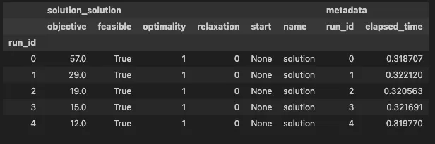

As shown above, using MINTO makes it easy to compare the results of optimization calculations for different numbers of machines. In the example above, you can see that the makespan (objective) decreases each time the number of machines increases. This is because increasing the number of machines allows for more efficient distribution of jobs. In this way, MINTO makes it easier to execute and manage optimization calculations and quickly analyze experimental results.