ソルバーによる求解 (OMMX)

このセクションでは、数理モデルに渡すインスタンスデータを定義し、さらに求解を行う処理を説明します。

インスタンスデータの定義

前の章ではJijModelingを使って、並列ジョブショップスケジューリング問題のモデルを定義しました。この時、ジョブの処理時間やマシン数などの具体的なデータはPlaceholderを使って定義しました。これらのPlaceholderに具体的な値を与えましょう。以下のように、インスタンスデータをPythonの辞書として定義します。


# インスタンスデータの定義
# Example: 10 jobs with their respective processing times
job_times_data = [5, 8, 3, 6, 9, 4, 7, 5, 2, 8]
# Example: 3 machines are available
num_machines_data = 3

# Prepare the data in the dictionary format required by JijModeling Placeholders
instance_data = {
    "JT": job_times_data,
    "M": num_machines_data,
}

続いて、このデータを前の章で作った数理モデルと組み合わせて、具体的なインスタンスを作成します。JijModelingのInterpreterを使って、Placeholderに具体的な値を与えたインスタンスを生成します。


# 1. Create an Interpreter to evaluate the problem with specific instance data
interpreter = jm.Interpreter(instance_data)
# 2. Evaluate the problem to create a concrete instance for the solver
instance = interpreter.eval_problem(problem)

ここで作成したインスタンスは、OMMXと呼ばれる数理最適化フォーマットとして表現されています。

OMMXとは何か：目的と利点

OMMX (Open Mathematical prograMming eXchange) は、数理最適化モデルを表現するためのオープンな標準ファイル形式、およびそれを操作するためのSDKです。JijModelingのようなモデリングツールで作成した最適化問題を、特定のツールや言語に依存しない共通の形式で保存・共有するために開発されました。

OMMXの主な特徴

相互運用性 (Interoperability): JijModelingで作成したモデルをOMMXの形式に変換し、多種多様なソルバーが使用可能なように変換することにより、ソルバーツール間の連携をスムーズにします。
永続性 (Persistence): 最適化モデルをファイル (.ommx) として保存できるため、後で再利用したり、他のユーザーと共有したりすることが容易になります。
共有とコラボレーション: 標準化されたフォーマットにより、チーム内や組織間で最適化モデルを簡単に共有し、共同で作業を進めることができます。
ツール非依存: モデルの定義が特定のモデリングツールに縛られないため、将来的にツールを乗り換える場合や、複数のツールを併用する場合にも柔軟に対応できます。

ソルバーを用いた求解

さて、作成したインスタンスをOMMXを使って解く例を見てみましょう。ここでは、OMMX形式から数理最適化ソルバーの一つであるSCIPを利用して解く方法を示します。 OMMX Adapterを使うことにより以下の二行のコードで完了します。


# Import the necessary adapter and interpreter
import ommx_pyscipopt_adapter as scip_ad
solution = scip_ad.OMMXPySCIPOptAdapter.solve(instance)

この二行のコードにて以下が行われています。

OMMX形式のインスタンスを、JijZept SDKのソルバーであるPySCIPOptに渡して解きます。
解が得られた後、OMMX形式のインスタンスから解を取得します。

さて、解いた結果を見てみましょう。以下のように、OMMXのsolutionから解を取得することができます。


import pandas as pd

optimal_makespan = solution.objective
print(f"
--- Solver Results ---")
print(f"Optimal Makespan: {optimal_makespan:.2f}")
assignment = {}  # {machine_idx: [job_idx, ...]}
assigned_jobs_flat = (
    []
)  # To store data for DataFrame: [{'Job': i, 'Machine': m, 'Time': t}]
x_result = {}

x_result = solution.extract_decision_variables("x")

# Process the extracted x_result dictionary
num_machines_instance = instance_data["M"]
for indices, val in x_result.items():
    # indices should be a tuple like (i, m)
    if len(indices) == 2 and val > 0.5:  # Check for binary '1'
        i, m = indices  # Unpack the indices
        if m not in assignment:
            assignment[m] = []
        assignment[m].append(i)
        # Ensure job index i is valid before accessing JT
        if 0 <= i < len(instance_data["JT"]):
            assigned_jobs_flat.append(
                {"Job": i, "Machine": m, "Time": instance_data["JT"][i]}
            )
        else:
            print(
                f"Warning: Invalid job index {i} found in solution variable 'x' for machine {m}."
            )

print("
Job Assignments per Machine:")
if assignment:
    for m_idx in range(num_machines_instance):
        assigned_jobs = sorted(assignment.get(m_idx, []))
        print(f"  Machine {m_idx}: Jobs {assigned_jobs}")
else:
    # This case might occur if x_result extraction failed or was empty despite optimal objective
    print("  No assignments could be extracted from 'x' variables.")

# Display assignments clearly using a Pandas DataFrame
if assigned_jobs_flat:
    assignment_df = pd.DataFrame(assigned_jobs_flat)
    print("
Assignment Details (DataFrame):")
    print(
        assignment_df.sort_values(by=["Machine", "Job"]).reset_index(
            drop=True
        )
    )
else:
    print("
Assignment Details (DataFrame): Empty")

以下のように出力されるはずです。


--- Solver Results ---
Optimal Makespan: 19.00

Job Assignments per Machine:
  Machine 0: Jobs [5, 7, 8, 9]
  Machine 1: Jobs [0, 1, 3]
  Machine 2: Jobs [2, 4, 6]

Assignment Details (DataFrame):
   Job  Machine  Time
0    5        0     4
1    7        0     5
2    8        0     2
3    9        0     8
4    0        1     5
5    1        1     8
6    3        1     6
7    2        2     3
8    4        2     9
9    6        2     7

また、結果の可視化を行うと次のようになります。


# Import plotting libraries if not already done
import matplotlib.pyplot as plt
import numpy as np
import pandas as pd  # For the DataFrame display (assuming done in Sec 9)

num_machines_instance = instance_data["M"]
num_jobs_instance = len(instance_data["JT"])
job_times = instance_data["JT"]  # Alias for convenience

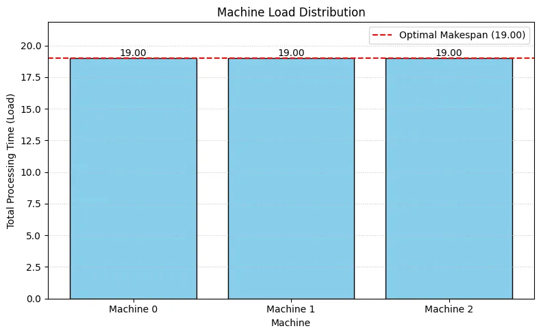
# --- Analysis: Calculate Machine Loads ---
print("--- Result Analysis ---")
print("Total Processing Time (Load) per Machine:")
machine_loads = {m: 0 for m in range(num_machines_instance)}
machine_load_list = []  # To store loads for plotting and verification

# Calculate loads directly from the 'assignment' dictionary
for m_idx in range(num_machines_instance):
    load = 0
    assigned_job_indices = assignment.get(m_idx, [])
    for job_idx in assigned_job_indices:
        if 0 <= job_idx < len(job_times):
            load += job_times[job_idx]
        else:
            print(
                f"Warning: Invalid job index {job_idx} found for machine {m_idx} during load calculation."
            )
    machine_loads[m_idx] = load
    machine_load_list.append(load)
    print(f"  Machine {m_idx}: {load:.2f}")

# --- Verification ---
calculated_max_load = max(machine_load_list) if machine_load_list else 0
print(f"Calculated Maximum Machine Load: {calculated_max_load:.2f}")
print(f"(Solver's Optimal Makespan: {optimal_makespan:.2f})")
# Use a small tolerance for float comparison
if abs(calculated_max_load - optimal_makespan) < 1e-6:
    print("-> Verification successful: Makespan matches the maximum machine load.")
else:
    print(
        "-> WARNING: Makespan does NOT match the calculated maximum load. Check model/solver."
    )

# --- Visualization 1: Bar chart of machine loads ---
print("--- Visualization ---")
plt.figure(figsize=(8, 5))
machines = [f"Machine {m}" for m in range(num_machines_instance)]
bars = plt.bar(machines, machine_load_list, color="skyblue", edgecolor="black")
plt.axhline(
    optimal_makespan,
    color="red",
    linestyle="--",
    label=f"Optimal Makespan ({optimal_makespan:.2f})",
)

for bar in bars:
    yval = bar.get_height()
    plt.text(
        bar.get_x() + bar.get_width() / 2.0,
        yval,
        f"{yval:.2f}",
        va="bottom",
        ha="center",
    )

plt.xlabel("Machine")
plt.ylabel("Total Processing Time (Load)")
plt.title("Machine Load Distribution")
plt.legend()
plt.grid(axis="y", linestyle=":", alpha=0.7)
plt.ylim(0, optimal_makespan * 1.15)
plt.tight_layout()
plt.show()

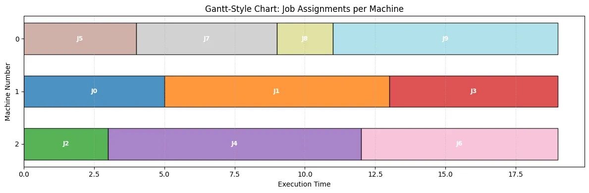
# --- Visualization 2: Gantt-Style Chart of Assignments ---
# This chart shows the jobs assigned to each machine sequentially.
# The horizontal axis represents time.
# Based on the user-provided snippet's logic.

fig, ax = plt.subplots(figsize=(12, max(4, num_machines_instance * 0.8)))
# Track the current end time for each machine
machine_end_times = np.zeros(num_machines_instance)
job_colors = plt.cm.get_cmap("tab20", num_jobs_instance)  # Distinct colors for jobs

print("Generating Gantt-style assignment chart...")

# Iterate through machines and the jobs assigned to them
for m_idx in range(num_machines_instance):
    # Get assigned jobs for this machine, sort for consistent plotting (optional)
    assigned_job_indices = sorted(assignment.get(m_idx, []))

    for job_idx in assigned_job_indices:
        if 0 <= job_idx < len(job_times):
            job_time = job_times[job_idx]
            start_plot_time = machine_end_times[m_idx]

            # Plot the bar for the job
            ax.barh(
                m_idx,
                job_time,
                left=start_plot_time,
                height=0.6,
                align="center",
                color=job_colors(job_idx % job_colors.N),
                edgecolor="black",
                alpha=0.8,
            )

            # Add job index text inside the bar
            # Adjust text position slightly for better visibility
            text_x = start_plot_time + job_time / 2.0
            text_y = m_idx  # Vertically center within the bar's height
            ax.text(
                text_x,
                text_y,
                f"J{job_idx}",
                va="center",
                ha="center",
                color="white",
                fontweight="bold",
                fontsize=9,
            )

            # Update the end time for this machine
            machine_end_times[m_idx] += job_time
        else:
            # This condition should ideally not be met if extraction worked
            print(
                f"Skipping plotting for invalid job index {job_idx} on machine {m_idx}"
            )

# --- Configure plot appearance ---
ax.set_xlabel("Execution Time")
ax.set_ylabel("Machine Number")
# Set y-ticks to match machine indices
ax.set_yticks(range(num_machines_instance))
ax.set_yticklabels(
    [f"{m}" for m in range(num_machines_instance)]
)  # Label ticks with machine numbers
ax.set_title("Gantt-Style Chart: Job Assignments per Machine")

# Improve appearance
ax.invert_yaxis()  # Show Machine 0 at the top
plt.grid(axis="x", linestyle=":", alpha=0.6)
# Set x-axis limit slightly beyond makespan for clarity
plt.xlim(0, optimal_makespan * 1.05)
plt.tight_layout()
plt.show()

以下のような出力となり、ソルバーで解いた結果が可視化できます。

次のセクションでは、MINTOを使用した計算の実行と最適化実行の管理について学びます。

次へ：最適化計算のベンチマーク、実験管理 (MINTO)

学習パス

習熟度レベル

数理最適化の基礎

リソースライブラリ

ソルバーによる求解 (OMMX)

インスタンスデータの定義

OMMXとは何か：目的と利点

OMMXの主な特徴

ソルバーを用いた求解