For v3 (previous version) product information, usage plans, and licensing, see the JijZept Solver v3 page.
v4 Beta: Early Access Trial Now Open
JijZept Solver
Mathematical Optimization Solver for Practical Problems
An optimization solver made by JIJ. It supports a wide range of problem classes, making it suitable for solving practical problems.

What Makes JijZept Solver v4 Different
Multiple engines run side by side, exchanging solutions
Three search engines with different characteristics work cooperatively, exchanging solutions.
Branch-and-Bound (B&B) Engine
Provides optimality guarantees
Constraint Programming (CP) Engine
Prunes candidates through logical inference
JIJ's Proprietary Heuristics
Structure-specialized search
▲▼ Exchanging solutions ▲▼
* Branch and bound = a search framework that can guarantee how close a solution is to optimal.
* Constraint programming = a method that prunes candidates through logical inference over constraints.
Supported Problem Classes
Automatically identifies the problem class and selects the optimal search method internally,
eliminating the need to be aware of problem characteristics.
- Linear Programming (LP)
- Mixed Integer Linear Programming (MILP)
- Quadratic Programming (QP)
- Quadratic Constrained Programming (QCP)
- Mixed Integer Quadratic Programming (MIQP)
- Mixed Integer Quadratic Constrained Programming (MIQCP)
v4 also supports "problem structure declaration"
In addition to problem classes, you can declare problem structures such as "tour route (TSP)" when solving. The range of supported structures will continue to expand.
Performance
Designed to return usable solutions within the time frame of real-world decision-making.
Feasible solutions from one second, even where commercial solvers return none
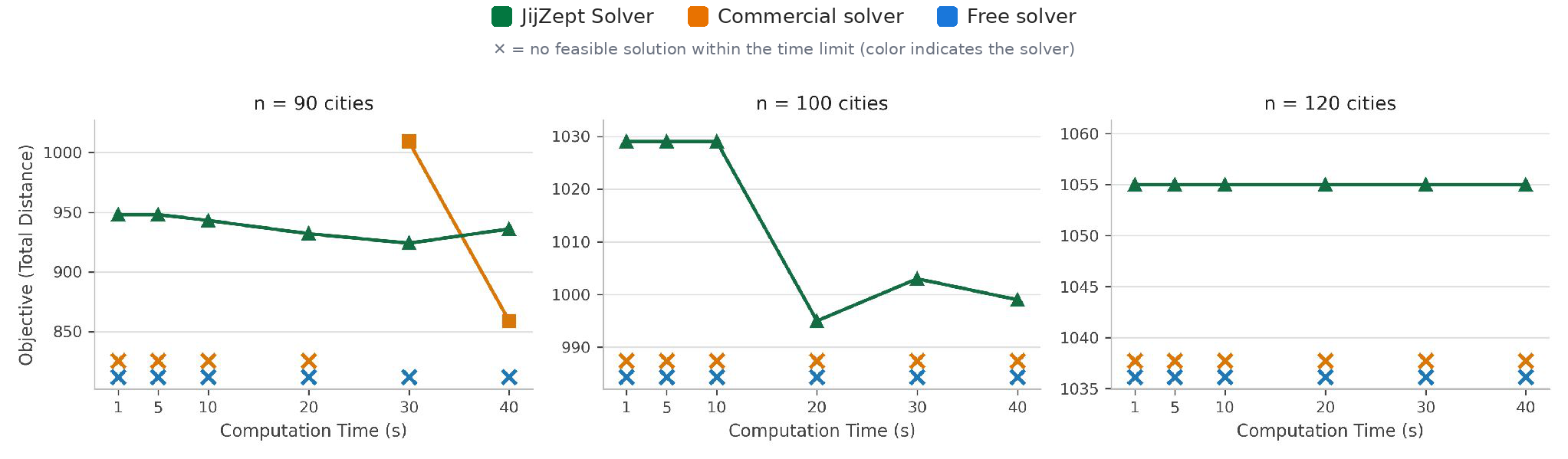
We compare existing commercial and free solvers with the new version on traveling salesman problems with time windows (TSPTW) of 90 to 120 cities. On 90 cities, the new version finds a feasible solution in 1 second versus 30 seconds for a commercial solver, and on 100 and 120 cities, only the new version obtains feasible solutions within the time limit.
Usable solutions within decision-making time on large real-world problems
Even on large problems from real operations, the new version returns solutions within the time available for decision-making. On a real problem with 160,000 variables where commercial and free solvers return no solution within the time limit, it is the only solver to obtain a feasible solution.
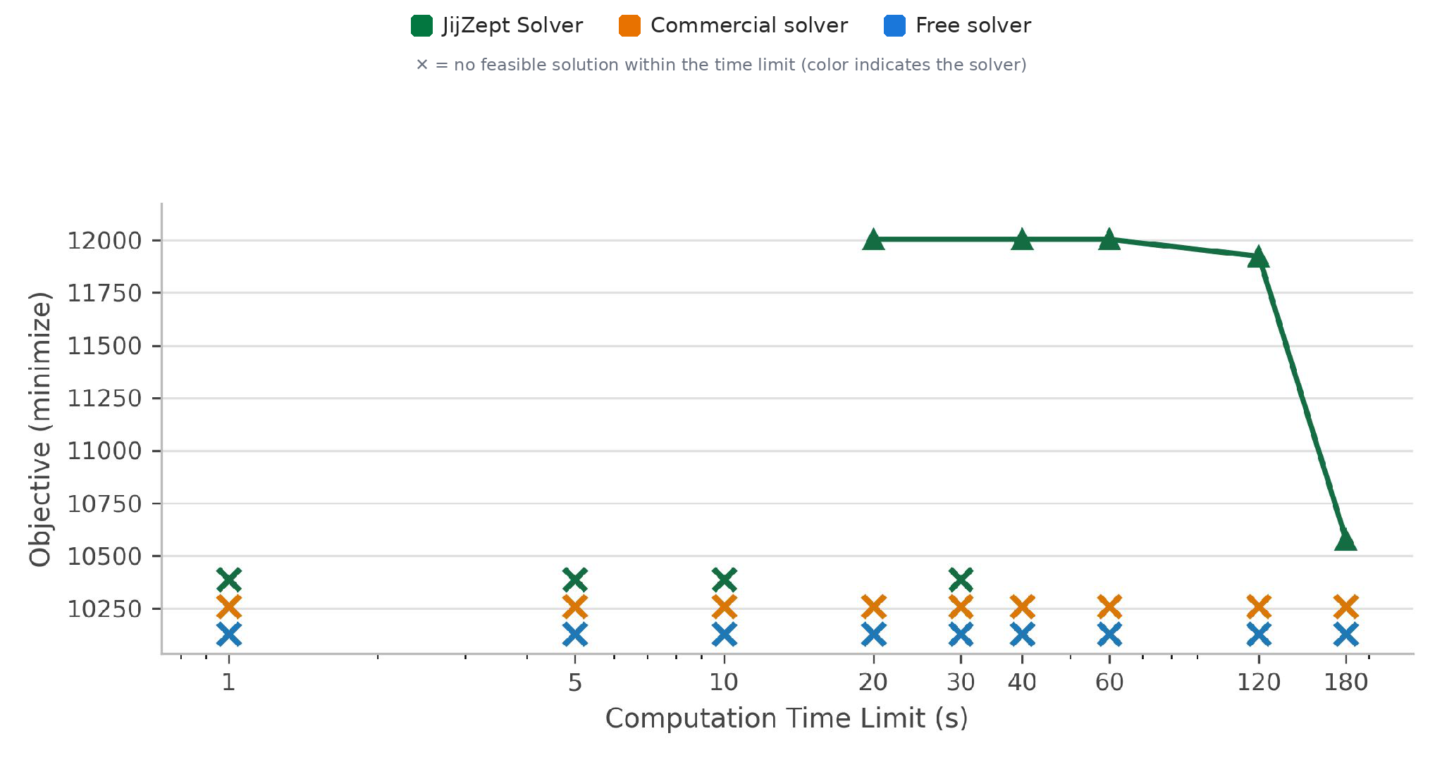
* Feasible solution = a solution that satisfies all constraints.
* TSPTW (traveling salesman problem with time windows) = deciding the visiting order when each location specifies an arrival time window.
* An ✕ in the charts indicates that no feasible solution was obtained within the time limit (the color of the ✕ indicates the solver).
* The TSPTW benchmark is measured with the problem structure declaration explicitly specified.
* Measured by JIJ (July 2026). The same problems were solved with each solver for comparison. Performance depends on the problem.
What's New Compared to JijZept Solver v3
The v3 algorithms are included in v4, so problems you solve with v3 can be solved as they are.
| Item | v3 | v4 |
|---|---|---|
| Search method | JIJ's proprietary heuristics | Cooperative parallel search combining branch and bound, constraint programming, and heuristics |
| Optimality gap reporting (an upper bound on how far the current solution can be from optimal) | None | Available (also for quadratic constraints and objectives) |
| Problem structure declaration | None | Available |
A large improvement in the feasible-solution rate
On a benchmark of 232 problems, the feasible-solution rate improves from 68.5% with the previous version to 82.8% with the new version (an improvement of 14.3 percentage points).
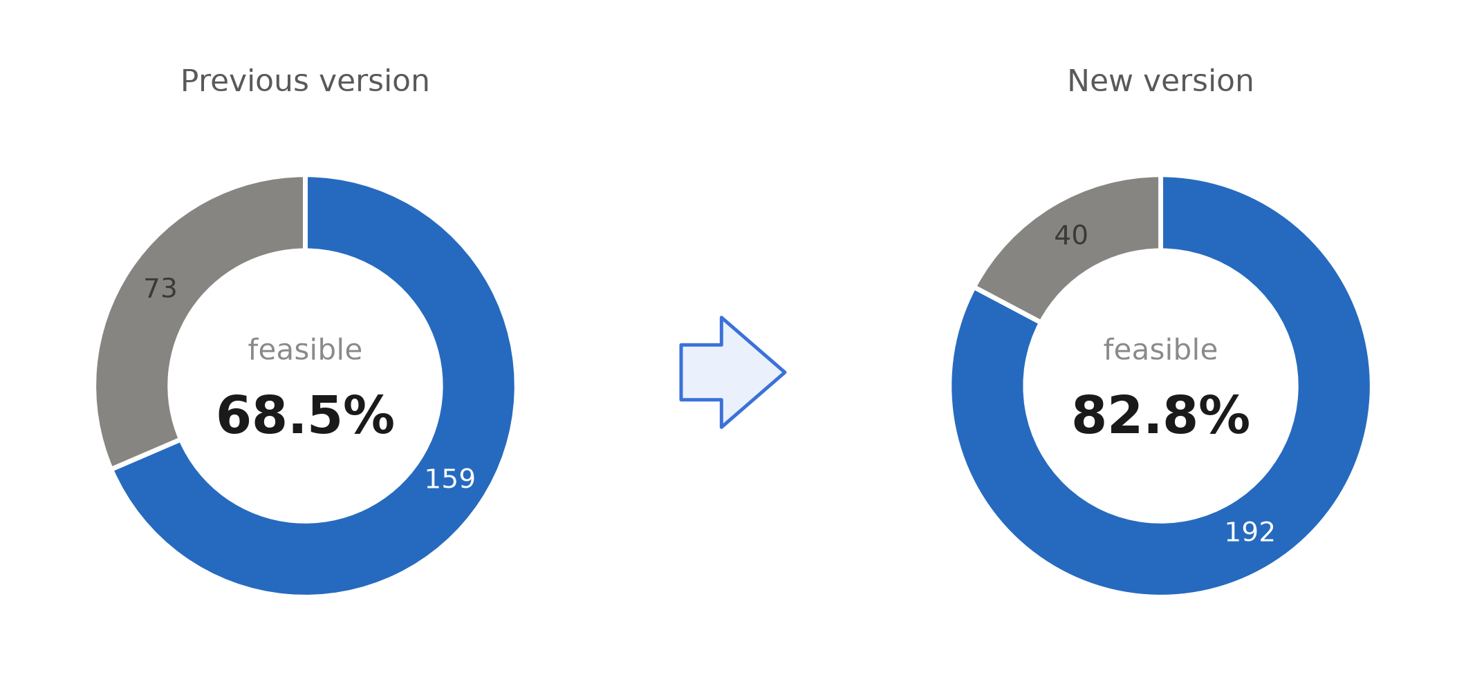
* Measured by JIJ (July 2026). The benchmark uses MIPLIB (a public library of mixed-integer programming benchmark problems).
To join the beta early access trial, please contact us.
A free Web API version is also available — no credit card required.
Here are the 4 steps to run JijZept Solver via the free Web API.
1 Application
Application
To use the JijZept Solver Free Web API, please first apply through the application form.
Free Use Application Form 2 Installation
Installation
Install the JijZept Solver Free Web API client package. Since the current release is a beta, add the --pre option.
pip install --pre jijzept_solver 3 Environment Variable Setup
Environment Variable Setup
Set the following values obtained through the application process as environment variables:
- JIJZEPT_SOLVER_SERVER_HOST: API server hostname
- JIJZEPT_SOLVER_ACCESS_TOKEN: Access token
Setup Examples
Environment variable setup example:
export JIJZEPT_SOLVER_SERVER_HOST='API server hostname'export JIJZEPT_SOLVER_ACCESS_TOKEN='Access token'Or example of setting within Python code:
import os
os.environ["JIJZEPT_SOLVER_SERVER_HOST"] = "API server hostname"os.environ["JIJZEPT_SOLVER_ACCESS_TOKEN"] = "Access token"
4 Solving Examples
Solving Examples
Since JijModeling is used in the examples, please install it in advance.
pip install jijmodelingUse the tabs below to switch between a knapsack example and a TSP example that uses a structure hint.
import loggingimport jijzept_solverimport jijmodeling as jm
logging.basicConfig(level=logging.INFO)
@jm.Problem.define("Knapsack", sense=jm.ProblemSense.MAXIMIZE)def knapsack(problem: jm.DecoratedProblem):    v = problem.Float(ndim=1)  # Item values    N = problem.NamedExpr(v.len_at(0))  # Number of items    w = problem.Float(shape=N)  # Item weights    W = problem.Float()  # Knapsack capacity    x = problem.BinaryVar(shape=N)  # Decision variables
    problem += jm.sum(v[i] * x[i] for i in N)  # Objective function: maximize value    problem += problem.Constraint("weight", jm.sum(w[i] * x[i] for i in N) <= W)  # Weight constraint
# Instance datainstance_data = {    "v": [10, 13, 18, 31, 7, 15],  # Item values    "w": [11, 15, 20, 35, 10, 33],  # Item weights    "W": 47,  # Knapsack capacity}
# Create OMMX instanceinstance = knapsack.eval(instance_data)
# Execute API requestsolution = jijzept_solver.solve(instance, time_limit=2.0)print(f"Value of the objective function: {solution.objective}")
import jijzept_solverimport jijmodeling as jm
# Distance data for 5 cities (large diagonal values keep self-loops out)num_cities = 5distances = [ [float(abs(i - j)) for j in range(num_cities)] for i in range(num_cities)]for city in range(num_cities): distances[city][city] = 1_000_000.0
@jm.Problem.define("TSP", sense=jm.ProblemSense.MINIMIZE)def tsp(problem: jm.DecoratedProblem): d = problem.Float(ndim=2) # Distances between cities N = problem.NamedExpr(d.len_at(0)) # Number of cities x = problem.BinaryVar(shape=(N, N)) # Whether to travel from city i to city j
# Objective function: minimize total travel distance problem += jm.sum(d[i, j] * x[i, j] for i in N for j in N) # No tour constraints here -- the structure declaration tells the solver
# Create OMMX instanceinstance = tsp.eval({"d": distances})
# Declare "x has the tour-route (TSP) structure" in one line and solvesolution = jijzept_solver.solve( instance, structure=jijzept_solver.Structure.tsp("x"), time_limit=10.0,)print(f"Total travel distance: {solution.objective}")
Each request to the free Web API can run for up to 10 seconds.
For longer runs (beta early access trial) or pre-benchmarks on your real data
(anonymized data accepted), please contact us.
Q.Can I try it for free?
Q.Can I try it for free?
Yes. The free Web API version is available without registering credit card information, and there is no limit on the number of applications.
Free Web API Q.Is there a limit on the number of requests?
Q.Is there a limit on the number of requests?
A.There is no limit. However, temporary access restrictions may apply if API requests from the same source are concentrated. In such cases, please wait and try again later.
Q.I was unable to get good solutions with the free Web API version.
Q.I was unable to get good solutions with the free Web API version.
You may get better solutions by setting the execution time (time_limit) to the maximum of 10 seconds, or by declaring the problem structure (structure). If that is not enough, consider the beta early access trial, which allows longer run times.
Contact Us Q.Does it support MPS files?
Q.Does it support MPS files?
A.Yes. You can load MPS files through OMMX's MPS loader, so any modeling tool that exports MPS files works — for example PuLP (a free modeling library widely used in Python).
Q.Can I check the progress during solving?
Q.Can I check the progress during solving?
A.With the on-premises version, you can check logs during computation, such as the progression of incumbent solutions.
Q.Can you provide specific pricing for on-premises deployment?
Q.Can you provide specific pricing for on-premises deployment?
Pricing varies depending on your requirements and scale. We provide quotes after understanding your challenges and needs. Please feel free to contact us first.
Contact Us